How do evalueate the definite integral

The definite integral generalizes the concept of the area under a curve. We lift the requirements that [latex]f(x)[/latex] be continuous and nonnegative, and define the definite integral as follows.

Definition

If [latex]f(x)[/latex] is a function defined on an interval [latex][a,b][/latex], the definite integral of [latex]f[/latex] from [latex]a[/latex] to [latex]b[/latex] is given by

provided the limit exists. If this limit exists, the function [latex]f(x)[/latex] is said to be integrable on [latex][a,b][/latex], or is an integrable function.

The integral symbol in the previous definition should look familiar. We have seen similar notation in the chapter on Applications of Derivatives, where we used the indefinite integral symbol (without the [latex]a[/latex] and [latex]b[/latex] above and below) to represent an antiderivative. Although the notation for indefinite integrals may look similar to the notation for a definite integral, they are not the same. A definite integral is a number. An indefinite integral is a family of functions. Later in this chapter we examine how these concepts are related. However, close attention should always be paid to notation so we know whether we’re working with a definite integral or an indefinite integral.

Integral notation goes back to the late seventeenth century and is one of the contributions of Gottfried Wilhelm Leibniz , who is often considered to be the codiscoverer of calculus, along with Isaac Newton. The integration symbol [latex]\displaystyle\int[/latex] is an elongated S, suggesting sigma or summation. On a definite integral, above and below the summation symbol are the boundaries of the interval, [latex][a,b][/latex]. The numbers [latex]a[/latex] and [latex]b[/latex] are [latex]x[/latex]-values and are called the limits of integration; specifically, [latex]a[/latex] is the lower limit and [latex]b[/latex] is the upper limit. To clarify, we are using the word limit in two different ways in the context of the definite integral. First, we talk about the limit of a sum as [latex]n\to \infty[/latex]. Second, the boundaries of the region are called the limits of integration.

We call the function [latex]f(x)[/latex] the integrand, and the [latex]dx[/latex] indicates that [latex]f(x)[/latex] is a function with respect to [latex]x[/latex], called the variable of integration. Note that, like the index in a sum, the variable of integration is a dummy variable , and has no impact on the computation of the integral. We could use any variable we like as the variable of integration:

[latex]\displaystyle\int_a^b f(x) dx=\displaystyle\int_a^b f(t) dt=\displaystyle\int_a^b f(u) du[/latex]

Previously, we discussed the fact that if [latex]f(x)[/latex] is continuous on [latex][a,b][/latex], then the limit [latex]\underset <\lim>\displaystyle\sum_^ f(x_i^*)\Delta x[/latex] exists and is unique. This leads to the following theorem, which we state without proof.

Continuous Functions Are Integrable

If [latex]f(x)[/latex] is continuous on [latex][a,b][/latex], then [latex]f[/latex] is integrable on [latex][a,b][/latex].

Functions that are not continuous on [latex][a,b][/latex] may still be integrable, depending on the nature of the discontinuities. For example, functions with a finite number of jump discontinuities on a closed interval are integrable.

It is also worth noting here that we have retained the use of a regular partition in the Riemann sums. This restriction is not strictly necessary. Any partition can be used to form a Riemann sum. However, if a nonregular partition is used to define the definite integral, it is not sufficient to take the limit as the number of subintervals goes to infinity. Instead, we must take the limit as the width of the largest subinterval goes to zero. This introduces a little more complex notation in our limits and makes the calculations more difficult without really gaining much additional insight, so we stick with regular partitions for the Riemann sums.

Example: Evaluating an Integral Using the Definition

Use the definition of the definite integral to evaluate [latex]\displaystyle\int_0^2 x^2 dx[/latex]. Use a right-endpoint approximation to generate the Riemann sum.

We first want to set up a Riemann sum. Based on the limits of integration, we have [latex]a=0[/latex] and [latex]b=2[/latex]. For [latex]i=0,1,2, \cdots ,n[/latex], let [latex]P=\[/latex] be a regular partition of [latex][0,2][/latex]. Then

Since we are using a right-endpoint approximation to generate Riemann sums, for each [latex]i[/latex], we need to calculate the function value at the right endpoint of the interval [latex][x_,x_i][/latex]. The right endpoint of the interval is [latex]x_i[/latex], and since [latex]P[/latex] is a regular partition,

Then the Riemann sum takes the form

[latex]\displaystyle\sum_^ f(x_i)\Delta x=\displaystyle\sum_^ (\frac)\frac=\displaystyle\sum_^ \frac=\frac\displaystyle\sum_^ i^2[/latex].

Using the summation formula for [latex]\displaystyle\sum_^ i^2[/latex], we have

Now, to calculate the definite integral, we need to take the limit as [latex]n\to \infty[/latex]. We get

Try It

Use the definition of the definite integral to evaluate [latex]\displaystyle\int_0^3 (2x-1) dx[/latex]. Use a right-endpoint approximation to generate the Riemann sum.

Hint

Use the solving strategy from the last example.

Try It

Evaluating Definite Integrals

Evaluating definite integrals this way can be quite tedious because of the complexity of the calculations. Later in this chapter we develop techniques for evaluating definite integrals without taking limits of Riemann sums. However, for now, we can rely on the fact that definite integrals represent the area under the curve, and we can evaluate definite integrals by using geometric formulas to calculate that area. We do this to confirm that definite integrals do, indeed, represent areas, so we can then discuss what to do in the case of a curve of a function dropping below the [latex]x[/latex]-axis.

Example: Using Geometric Formulas to Calculate Definite Integrals

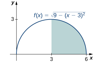
Use the formula for the area of a circle to evaluate [latex]\displaystyle\int_3^6 \sqrt dx[/latex].

The function describes a semicircle with radius 3. To find

we want to find the area under the curve over the interval [latex][3,6][/latex]. The formula for the area of a circle is [latex]A=\pi r^2[/latex]. The area of a semicircle is just one-half the area of a circle, or [latex]A=(\frac)\pi r^2[/latex]. The shaded area in Figure 1 covers one-half of the semicircle, or [latex]A=(\frac)\pi r^2[/latex]. Thus,

[latex]\begin \displaystyle\int_3^6 \sqrt & =\frac\pi (3)^2 \\ & =\frac\pi \\ & \approx 7.069. \end[/latex]

in quadrant one over the interval [0,6] with center at (3,0). The area under the curve over the interval [3,6] is shaded in blue." width="325" height="200" />

Figure 1. The value of the integral of the function [latex]f(x)[/latex] over the interval [latex][3,6][/latex] is the area of the shaded region.

Watch the following video to see the worked solution to Example: Using Geometric Formulas to Calculate Definite Integrals.

For closed captioning, open the video on its original page by clicking the Youtube logo in the lower right-hand corner of the video display. In YouTube, the video will begin at the same starting point as this clip, but will continue playing until the very end.

Try It

Use the formula for the area of a trapezoid to evaluate [latex]\displaystyle\int_2^4 (2x+3) dx[/latex].

Graph the function [latex]f(x)[/latex] and calculate the area under the function on the interval [latex][2,4][/latex].